Shape memory alloys (SMA) exhibit a highly temperature-dependent stress-strain behaviour. It is characterized by large, recoverable strains. Furthermore, the stress-strain relation is hysteretic, thus the material behaviour is highly non-linear. It is well-known that the macroscopic behaviour of these alloys is based on a solid-solid phase transition of the metallic lattice: At high temperatures and in the absence of a load, a symmetric cubic lattice is stable , which is called the austenitic lattice. This lattice may transform into sheared variants, which are less symmetric and create the martensitic lattice. The shear transformation involves large shear strains, and it may occur under the influence of external loads as well as under a change of the temperature: The austenite becomes unstable, if the temperature is lowered below a certain critical temperature and a martensitic lattice is created.
The macroscopic model by Mueller, Achenbach and Seelecke is based on the idea that it is macroscopic crystal layers that undergo the phase transition. A non-konvex energyfunction is postulated and statistical arguments are evaluated in order to find the thermodynamic equation of state of the body as a whole. This has led to a thermodynamic description, and the reader may test a java simulation that uses the model.
The question has arisen, how the shape memory effect may be expained by the interaction of the atoms that create the metallic lattice. To answer this question, a molecular dynamic model has been developed, and it shall be documented here. Everything will be explained in a paper of which this presentation is a preliminary draft.
It has turned out, that it is possible to simulate an austenite-to-martensite phase transition by molecular dynamics in the 2 D case. The following well-known effects can be simulated:
Lennard-Jones potential functions are employed to calculate the atomic interactions.
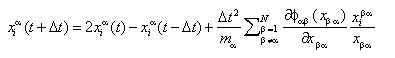
In molecular dynamics, the motion of N particles is calculated by the evaluation of the equations of ballance of the particles. We shall restrict the attention to the classical case. In order to keep the model as simple as possible only motion in two-dimensions is considered.
The N particles may belong to two types of atoms. Their motion is calculated by use of the Stoermer-Valet-algorithm:
This iteration scheme provides the positions of the particles alpha at timestep (t+Delta t), if the current positions (time t) and the positions at the previous timestep (t-Delta t) are known.
On the right hand side we find the interaction-term, expressed as the field of a potential function, that may be given by a two-parameter Lennard Jones potential, as shown below:
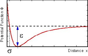
The interaction-parameter sigma determines the position of the potential well, while epsilon represents its depth. All particles interact with each other.
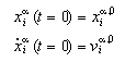
Two initial conditions must be given for each particle. They provided the set of inital positions and the set of initial velocities:
We are looking for a crystal configuration of particles in two dimensions that may undergo a solid-solid phase transition. Hence it is required that the particles do possess more than one configuration that is stable. Although interactions of all particles are allowed, we may find an initial guess of the positions by the consideration of nearest and next-nearest neighbours only: We may suppose a configuration being stable, if nearest and next nearest neighbours located in the potential wells of their potential functions. At these positions the interaction-force between pairs vanishes, hence the pair is supposed to be stable. Whether a configuration is stable or not has to be found from a dynamic simulation. It turnes out that this method leads to acceptable sets of initial positions.
In the following we shall discuss some possible configurations and their stability. Therefore we distinguish two cases: The case of one type of atoms, and the case of two types of atoms.
One type of atoms. If only one type of atoms is taken into account, we have only one Lennard-Jones-potential, and thus -- evaluating the foregoing idea-- we find that the crystal lattice is stable, in which neighbouring particles have all the same distance. Thus a hexagonal lattice as shown below is stable.
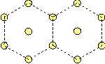
It is the only possibility to create a stable initial lattice, while it is impossible to create a stable square lattice for one type of atoms, since in a square lattice not all next neighbours possess the same distances!
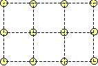
Two type of atoms. However, if we take into account two type of atoms, the cubic lattice may be stabilized. By placing the red atoms into the centers of the yellow squares, the cubic lattice becomes stable:
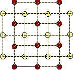
In the two-component-case there are three Lennard-Jones-potentials, one for each type of pairs (red-red, yellow-yellow, red-yellow). Hence there are six interaction parameters that may be chosen so as to stabilize the cubic lattice. This lattice is very symmetric and it consists of square unit cells. Therefore we may call this configuration the austenite. Furthermore, the two-component cubic lattice has the possibility to transform into sheared variants, and these are also stable:
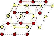
The sheared configuration consists of rhombic unit cells. It has lower symmetry than the square, and therefore we may call it the martensite. We observe hexagonal ring structures which are created by each component forming this lattice. Thus we may call the sheared lattice hexagonal.
The initial set of velocites is chosen randomly in orientation, but at equal speeds.By prescribing the initial speeds of the particles it it possible to fix the initial temperature of the crystal lattice, since the temperature is a measure for the mean kinetic energy of the particles.
-> Next page: Simulations
-> Top