- Change of temperature: Temperature -Control
- Application of external forces: Load-Control
- Prescription of positions of some chosen atoms: Displacement-Control
-> Back to previous page
-> Go directly to results
-> Table of contents
The procedure of a simulation experiment follows the scheme given below:
Temperature is proportional to the mean kinetic energy of an atom. Thus, if the temperature is "high", the atoms move quicker. Changing the temperature means changing the atomic velocities. However, the velocities are not directly computed, rather the Stoermer-Valet-algorithm provides positions. Thus the velocities must be calculated from the displacements

of the atoms over a time step: They may be found as

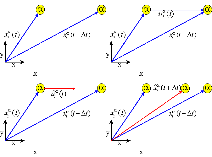
In order to slow down or accelerate the atoms, we may multiply the displacement vector u i by a factor k smaller or greater than 1,

and consequently re-calculate the new positions of the atoms by use of the shortened / enlonged displacement vector:
Thus, cooling or heating maybe controlled by the choice of the factor k. k=1 is the adibatic condition.
The following picture visualizes this idea of thermal annealing:

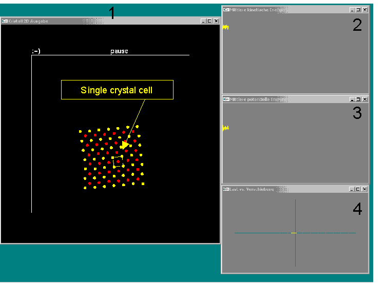
The simulation program permits the study of the austenitic-martensitic phase transformation on a display screen. The simulation program offers 4 windows shown below. Explanation may be found below this image.

Explanation of the windows 1 through 4:
| Window 1: | In the main window the motion of the atoms may be observed over time. Here one can see a block of 85 atoms of types "red" and "yellow" in a square (austenitic) lattice. |
| Window 2: | Kinetic energy versus time. |
| Window 3: | Potential energy versus time. |
| Window 4: | Ordinate: External force or reaction force as exerted on the uppermost row of atoms. Abscissa: Diplacemant of the atoms in the uppermost row from their initial configuration. This is of interest in load- or displacement controlled simulations only. |
In order to present some simuations here you may select an example from links listed below. Each link points to a result-page, where the observable phenomena are discussed. gif-file animations may be downloaded, which permit to study the progress of the simuations over time.
The following examples are represented: