This page provides some background information about
- the SMA model used for the simulations, and
- the numerical implementation of the model.
The SMA model. The following section gives a short overview of the SMA model used for the simulation page. It has originally been developed by Achenbach and Müller (1982, 1985) and Achenbach (1989) and has recently been modified by Seelecke (1999) in order to make quantitative predictions, see Seelecke (2000) and Seelecke and Kastner (2000) for details. It uses ideas from statistical thermodynamics and describes the evolution of two martensite fractions based on the theory of thermally activated processes.
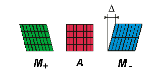
Under uniaxial loading conditions, three different phases can be observed in a shape memory alloy, viz. the austenite phase A and two martensitic twin variants M± , see Fig. 1 below:
 .
.
Figure 1: Lattice particle in different phases.
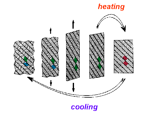
From crystallographic observations it is known that a macroscopic body under uniaxial loading forms a layered structure, each layer being in one of the three above phases. Motivated by this observation, we construct the model body according to Fig. 2.

Figure 2: SMA body under tensile loading/unloading at low temperature, exhibiting the shape memory effect upon heating.
The sequence in Fig. 2 shows the unloaded body at a low temperature on the left, at which the layers are in the martensitic state with an equal amount of each twin variant (green and blue). Under a tensile load, the M+-layers become flatter, while the M--layers become steeper (second from left), until the M--layers flip over to the M+-phase at a critical load (center). When the body is unloaded, the layers remain in the M+-phase, and a residual deformation results (second from right). Upon the supply of heat, the layers transform into austenite (red), and the body seems to remember its former shape, which gives the name to the effect (right). Subsequent cooling causes the austenitic layers to retransform into martensite with an equal probability for both twins to occur, and the original zig-zag shape of the surface is restored as well.
The basic idea to model this behavior is to assume that the phase transition
of the layers is a thermally activated process. The shear length ![]() of the layers fluctuates due to the thermal activation, and the layers
move in an energy landscape with load- and temperature-dependent barriers.
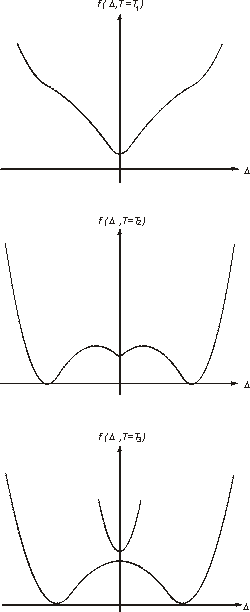
The relevant effective potential energy for a layer is given by the Gibbs
free energy, or, if there is no load, by the Helmholtz free energy. These
are nonconvex functions of the shear length with potential wells corresponding
to each phase, see Figure 3 below.
of the layers fluctuates due to the thermal activation, and the layers
move in an energy landscape with load- and temperature-dependent barriers.
The relevant effective potential energy for a layer is given by the Gibbs
free energy, or, if there is no load, by the Helmholtz free energy. These
are nonconvex functions of the shear length with potential wells corresponding
to each phase, see Figure 3 below.
 |
|
|
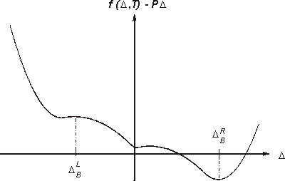
Figure 3: Effective potential energy functions of a layer: Helmholtz free energy (left) at three different temperatures (T1>T2>T3 ) and Gibbs free energy (right) at an intermediate temperature for a tensile load.
The rate of change of the phase fractions is given by the following equations
,
with transition probabilities
that can be calculated from statistical thermodynamics, e.g.
.
The above transition probability is given by the product of an inverse relaxation time
and the probability to find a layer on top of the Gibbs free energy barrier between the M--well and the austenite well.
The temperature T follows from the balance of internal energy for the SMA specimen,
,
relating the rate of change of temperature to heat exchange with the environment at temperature T0 and to the rate dependent release or absorption of latent heats. The latent heats are given by the last two terms on the RHS of Equation (3); they are determined by the differences in enthalpies of the phases. c and
are specific heat and heat exchange coefficient, respectively.
The system of ordinary differential equations in time (1) and (3) permits to calculate phase fractions and temperature for given initial conditions provided the loading function P(t) and environmental temperature T0(t) are known. The total deformation D of the SMA body follows from the fact that it is the sum of the deformation of all layers
.
Equation (4) can be considered as a load-deformation relation, because the mean values of the deformation in the individual phases depend on the load through the Gibbs free energy. They can again be calculated from statistical thermodynamics, e.g.
.
The Gibbs free energy from Fig. 3 is represented by a train of smoothly connecting convex and concave parabolae. Thus, the integrals in Eq. (5) can be solved analytically and the load-deformation relation (4) can be inverted, which is the basis for the simulation of a deformation-controlled experiment or for a finite element implementation.
Numerical implementation. From the preceding section, it becomes clear that the mathematical structure of the model is given by the system of nonlinear ordinary differential equations in time (1) and (3) and the algebraic relation (4). For the numerical solution of this system it is important to observe that it exhibits an extreme numerical stiffness, and hence, it is necessary to resort to implicit methods for a stable solution. For our FORTRAN implementations of the model, we rely on the RADAU5 routine by Hairer and Wanner. This routine uses an implicit Runge-Kutta method based on the Radau-IIa scheme, and it has proved to be very efficient for the solution of our system. The FORTRAN code is freely available at Ernst Hairer's homepage, and the algorithm is described in detail in an excellent textbook, Hairer and Wanner (1991).
For the JAVA version of our model we first tried to use simpler algorithms like implicit Euler or generalized midpoint rule schemes, but their performance was far from acceptable. Considering the fact that the interpreter language JAVA itself is already slower than FORTRAN, it is a definite matter of concern to have an efficient solution algorithm so that the user does not have to wait unreasonably long for the simulation output.
We finally ended up porting the RADAU5 routine to JAVA - and we were positively surprised about the speed of the calculation!It should be acknowledged here that we greatly benefitted from the FORTRAN original by Hairer and Wanner, which not only implements the Radau-IIa scheme, but features a "bag o' tricks" that really makes the code efficient.
References
Achenbach M (1989), A model for an alloy with shape memory, Int J Plast 5, 371--395.
Achenbach M and Müller I (1982), A model for shape memory, J de Phys Colloque C4 supplement au no 12, 163--167.
Achenbach M and Müller I (1985), Simulation of material behavior of alloys with shape memory, Arch Mech 37, 573--585.
Hairer E and Wanner G (1991), Solving Ordinary Differential Equations, II. Stiff and Differential-algebraic Problems, Springer Series in Computational Mathematics, Springer-Verlag.
Seelecke S (1999), Adaptive Structures with SMA Actuators - Modeling and Simulation (in German), Habilitation thesis, TU Berlin
Seelecke S (2000), A fully coupled thermomechanical model for shape memory alloys, Part I: Theory, in preparation.
Seelecke S and Kastner O (2000), A fully coupled thermomechanical model for shape memory alloys, Part II: Numerical simulation, in preparation.
