How to ...
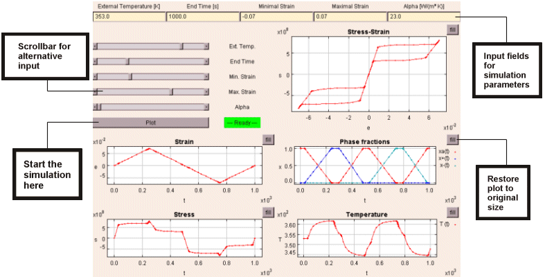
... use this simulation page? It is designed in a rather self-explanatory way and most of its contents will be instantaneously clear to you. Just fill in the parameter fields and press the Plot button, see the picture below. However, a few things are not so obvious, and it might be useful to browse through this section if this is your first time here. Also, you might find some inspirations for experimental phenomena that you want to simulate.

Parameter input.
For simulation of material behavior a model usually requires a large number
of parameters, which define the constitutive properties or fix initial
conditions. These parameters allow the model to be taylored to different
loading conditions and different materials, and of course, the more parameters
can be controlled, the more flexibly the model may be used. However, as
this page is the first time we offer the opportunity for an on-line simulation
of SMA behavior, we have restricted the possibilities a little. We have
confined the number of user-controllable parameters to those necessary
to define a typical experiment run in the laboratory, a deformation-controlled
tension/compression experiment. Also, all material data are fixed to represent
a typical NiTi specimen. Yet, you will see that there is still a large
number of interesting experiments that may be simulated demonstrating
the complexity of SMA behavior.
Deformation.
The deformation is given by a linearly ramped function in time. You can
set the values for different maximal positive and negative deformation,
thus allowing for unsymmetric and incomplete hysteresis loops.
Experiment duration. You can set the end time of the experiment,
which permits - together with the above extremal values of deformation
- a control of the deformation rate. You will observe that the hysteresis
loops are quite rate sensitive as a the result of the strong thermomechanical
coupling typical for shape memory alloys. Depending on the heat exchange
with the environment, the rate-dependent release or absorption of latent
heats of phase transformation may lead to self-heating or self-cooling
of the specimen. A suitable choice of parameters will permit you to observe
the complete range from isothermal to near adiabatic behavior.
Environmental
temperature. The environmental temperature can be set between
273K and 373K, such that for the implemented NiTi behavior the continuous
spectrum of load-deformation curves from quasiplasticity to pseudoelasticity
may be simulated.
A remark is necessary for experiments between 277 K
and 303 K. Below and above these temperatures the material is either purely
martensitic or purely austenitic in the unloaded state (this can be verified
by looking at the phase fraction plot). In the intermediate range, however,
the initial state of the material is not unique and depends on the prior
treatment. In order to perform the simulation with well-defined parameters,
we have implemented the following procedure:
-
heating of the unloaded specimen to a temperature of 373 K, where the material is austenitic, and
-
subsequent cooling to the prescribed environmental temperature.
This procedure, which would also have to be performed in a real experiment, is invisible to the user and is simulated before actual plotting starts.
Heat exchange cofficient. The heat exchange coefficient can be varied within a wide range in order to simulate different surrounding media like still or flowing air, oil, water etc..
Output. The output is arranged in five different diagrams. Below the alternative input area (scrollbars) you can see the prescribed deformation, and at the bottom, the stress in the specimen is plotted as a function of time. The two diagrams on the lower righthand side show the phase fractions and the temperature evolving in time. The load-deformation plot is shown on the right of the scrollbars . It exhibits the hysteresis loops typical for shape memory alloys.
Zooming. For a detailed view it is possible to zoom into each plot. You have to click and hold the left mouse button to span a rectangle by moving the mouse. Releasing the left mouse button then zooms into this area. To zoom out use the right mouse button. An alternative method is to use the 'fill' button beside each plot, which restores the original diagram.
Acknowledgement.
All the plotting and viewing capabilities of this simulation page rely
on PtPlot 3.1,
a JAVA-based plotting library developed at UC Berkeley.